|
|
Head tracking is important for several application in computer vision,
like 3D animation systems, virtual actors, expression analysis, face
identification and surveillance systems. Head motion can be used for
recognition of simple gestures, like head shaking or nodding, or for capturing
a person’s focus of attention, providing a natural cue for human machine
interfaces. Also for videoconferencing, encoding the head motion of the speaker
according to known standards, like MPEG4 compliant Facial Animation Primitives
(FAPs), allows to produce very low bit rate data streams. Many of these
applications calls for non intrusive and robust reconstruction techniques from
monocular views.
Our
approach to head tracking uses a textured 3D head model which is fitted to an
image sequence acquired using a single and non-calibrated camera. The model is
defined by a polygonal mesh. Fitting process exploits both motion and texture
information. Motion information is obtained evaluating the optical flow between
two consecutive frames, while texture information is gathered warping the image
frame in the texture space of the model. Minimization is achieved applying a
steepest descent based algorithm.
After
pose reconstruction, each input image is projected on the texture map of the
model. The dynamic texture map provides a stabilized view of the face which can
be used for further processing tasks, like facial expression analysis and
recognition.
In
the following sections we will outline the various components of the proposed
system.
The
model
Our
system uses an elliptical model defined by a polygonal mesh (see Fig. 1). This model is not able to
reproduce head features, like nose, mouth or accurate face profiles, but allows
fast computation and can be easily calibrated according to the user. However,
any other polygonal model can be used, regardless its complexity.
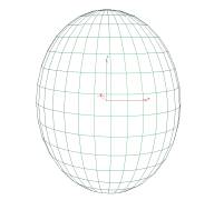
Fig. 1: face model
Model
motion
The
head is a rigid object and has six degrees of freedom (DOF). The first three
DOF define the translation of the model. The last three DOF describe the
rotations around the x, y and z axes. Therefore, each pose is determined by a vector à containing six values:
à = [tx ty tz rx
ry rz]
The
projection of the vertices of the model on the image plane is defined by a
transformation matrix G(Ã) written in homogenous
coordinates. An example of the final result of the transformation applied to
the model can be seen in Fig. 2.
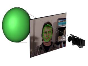
Fig. 2: projection of
the model on the image plane
Pose
reconstruction
The
reconstruction problem involves finding for each frame n the vector Ãn which minimizes the differences between model
and image features. Those discrepancies are described by an error function E which comprises motion and texture
errors. Minimization is obtained applying a steepest-descent based algorithm.
The
various components of the error function are detailed in the following
sections.
Motion
error
Here,
the main idea is to match the motion of the model with the corresponding
optical flow evaluated from two consecutive images. The optical flow at each
point (x,y) of the image is the
vector [u,v] which describes the translation of the pixel from the previous
image. We can also estimate the model flow as the translation on the image
plane of the model vertices, that is the difference between the positions of
the projected points between pose Ãn and candidate pose Ãn+1. Since not all the points are visible for both poses, this evaluation
must be computed only for the subset of common visible points. Let Vn and Vn+1 be the two subsets, and [uM,i,vM,i]
the i-th point estimated displacement
vector.
Optical
flow is evaluated using a pyramidal version of the Lucas-Kanade algorithm.
Texture
error
The
idea, again, is to match model and image features, that is the texture map
values associated to the projected model points and the values of the current
frame. These values are intensity values for achromatic images and RGB triples
for color images.
Combining
error functions
To
combine motion and texture information, the target error function is a weighted
sum of the corresponding error functions. The purpose of the weights is to
equalize the contribution of the different sources of information.
Finding
the optimal pose
Given
the error function E, we have to find
the pose which minimizes the discrepancies between model and image features.
The minimization of the function is obtained applying a steepest-descent based
method. The method is iterative and for each iteration the function values
corresponding to translations of ±dt and rotations of ±dr for x, y and z are evaluated.
The transformation giving the best improvement of the error value is selected
for the next iteration. When no improvement can be obtained, the values of dt and dr are reduced by a factor two and the process is iterated. The algorithm
is stopped when the deltas are lower than a predefined threshold or a maximum
number of iterations has been performed. In order to cope with large head
motion we apply an head motion estimation procedure on each frame of the
sequence before the error function minimization begins. The motion estimation
works as follows. A 2D translation vector, given by the mean value of the
optical flow of the visible model points, is evaluated in the image plane. This
translation vector is projected on the plane passing through the center of the
object and parallel to the image plane (see Fig. 3). The 3D vector obtained is
used as initial translation of the model.
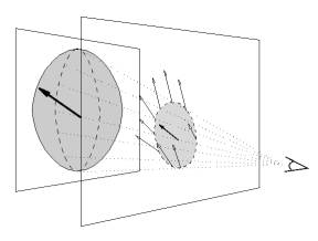
Fig. 3: head motion
estimation
Image
warping
When
the optimal pose has been found, the content of the current image is warped
into the texture map of the model. The warping function is the inverse of the
texture mapping function. The warped image produces a stabilized view of the
face, which can be used for further processing, like face expression analysis
and reconstruction.
Some
results of the tracking process can be seen in Fig. 4, where the input image, the
reconstructed posture and the dynamic texture are shown for several frames.
Inizialization
The
reconstruction process needs to know with a good precision the initial position
and orientation of the model. So far, this step requires user intervention to
align the face model to the head in the video images and to modify the size of
the model.


Fig. 4: results of
tracking on several frames of a test sequence,
including original image
(first column),
superimposed reconstructed
pose (second column) and dynamic texture map (last column)
In
order to perform a quantitative analysis of the performances of our system, we
have tested the described approach on several input video sequences. Each
sequence contains 200 frames whose size is 320×240
pixels. The data used show different performers and typical head movements,
including large head translation and rotation. Ground truth for position and
orientation of the head for each sequence have been acquired using a magnetic
sensor. Those sequences are available by courtesy of the Image and Video
Computing Group of the Boston University.
Only
the rotational values of the ground truth data have been used for comparison
with our results. As a matter of facts, the translation values refer to the
location of the magnetic marker, which is placed on the back side of the head.
Since in most of the sequences the marker itself is completely hidden we have
no way to guess its position with a sufficient precision.
The
reconstruction looks very stable for xyz
translation and for rotation around z
axis, while the system error increases when reconstructing large head rotations
around x and y axes. This is due to the fact that translation in the xy plane and x or y rotations produce
similar effects in the image plane. Another drawback is that, for large x and y rotations, the discrepancies between head profile and ellipsoidal
model become relevant. Better results might be obtained using synthesized
head-like surfaces. We are currently investigating this point.
Results
are plotted in Table 1 for several input
sequences. The first three columns show the mean reconstruction error in
degrees for rotations around x, y and z axes, while the last three columns show the maximal
reconstruction error for all the sequences. As can be seen the best average
results range between 1.32 and 2.76 degrees. It should be noted, however, that
the mean errors on x and y increase drastically when the sequence
analyzed contains large and fast variations of their values (as can be seen for
sequences Jam 5, Jam 6, Jam 7 and Jam 8). On the contrary, all the sequences
where z rotation is conspicuous are
reconstructed with good precision (such as Jam 1 and Jam 9). This observation
is also underlined by the fact that the worst average reconstruction error for z value does not exceed 4 degrees.
|
Seq. |
X |
Y |
Z |
X max |
Y max |
Z max |
|
Jam 1 |
1.87 |
2.76 |
2.85 |
5.32 |
9.07 |
11.17 |
|
Jam
2 |
2.34 |
7.84 |
2.26 |
6.17 |
26.47 |
5.36 |
|
Jam
3 |
1.81 |
5.83 |
1.71 |
6.71 |
9.74 |
5.37 |
|
Jam
4 |
2.79 |
7.05 |
3.72 |
6.73 |
12.08 |
9.03 |
|
Jam
5 |
3.12 |
14.90 |
2.00 |
7.39 |
34.07 |
7.15 |
|
Jam
6 |
12.12 |
3.06 |
2.85 |
25.58 |
7.49 |
9.59 |
|
Jam
7 |
1.32 |
10.73 |
2.23 |
4.78 |
21.65 |
6.61 |
|
Jam
8 |
4.22 |
10.02 |
3.44 |
19.64 |
31.75 |
13.90 |
|
Jam
9 |
3.83 |
5.30 |
3.05 |
11.06 |
12.65 |
9.67 |
Table 1: mean and
maximal angular reconstruction errors in degrees
Concerning
reconstruction time, the current implementation runs at about 15 frame/sec on a
Pentium III 500 Mhz. This value is nearly constant for all the tested sequences
despite the iterative nature of the reconstruction algorithm. It should be
noted, however, that the code is not optimized and the reconstruction time
includes also the time spent in reading and decoding the video stream.
Discarding acquisition time, the mean reconstruction rate is about 30
frame/sec. Considerable improvements can be expected exploiting graphical
hardware, like OpenGl accelerators, to perform model transformation and image
warping, which account for 20% of the execution time.