Home page gallery

Details

Last Updated on Friday, 23 January 2015 12:29

This page shows the figures which appear in the home page slideshow with a short description:

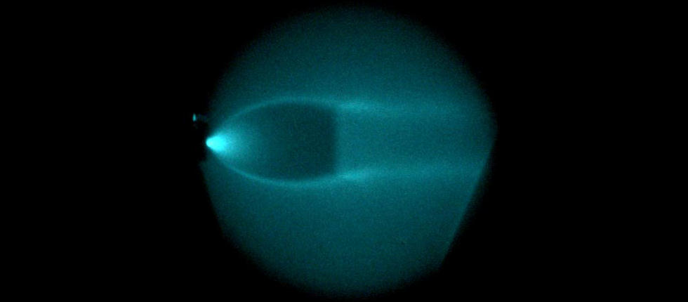
	Underexpanded jet, Ar/He, laboratory experiment.
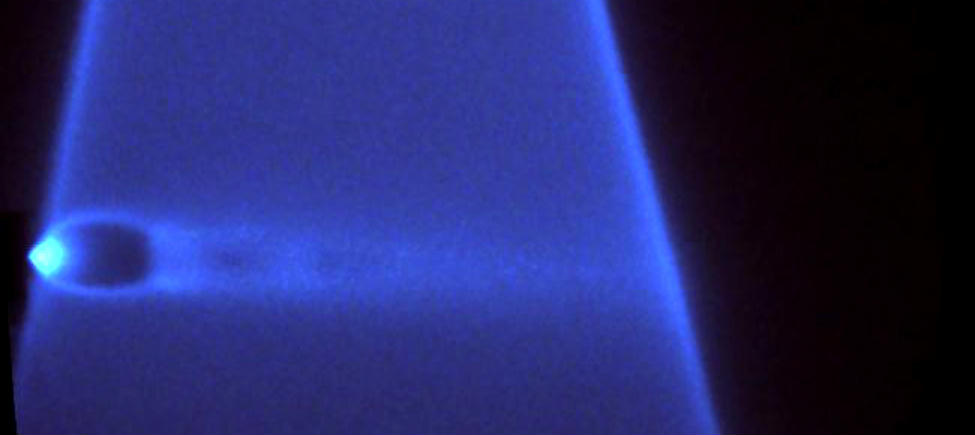
	He/Ar jet after 80 ms, laboratory experiment
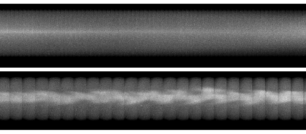
	Caption
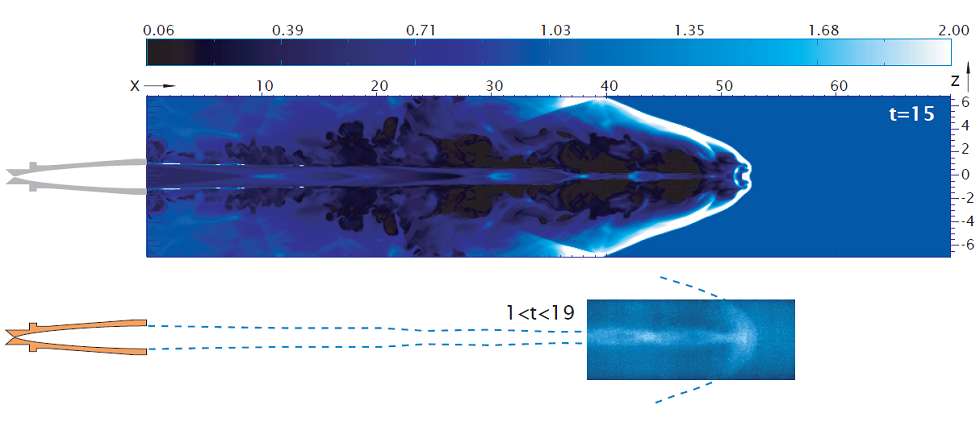
	He/Xe jet after 15 ms, numerical simulation
	He/Xe jet after 30 ms, numerical simulation
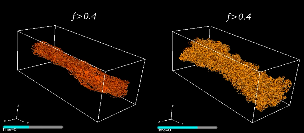
	Large-eddy simulation of a hypersonic light jet at M=5. The figure shows the underresolved regions where the small scale indicator f is larger than the threshold 0.4 at the dimensionless times 18 and 28 (see Tordella et al., Comput. Phys. Comm. 141, 2007).
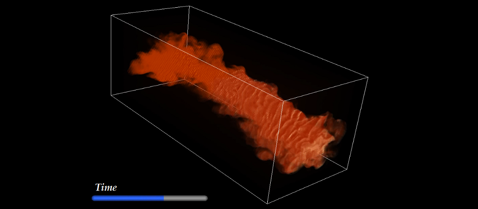
	Large-eddy simulation of an hypersonic light jet at M=5. The figure shows a passive tracer introduced at t=0 in the initially round jet after 28 sound crossing times. (see Tordella et al., Comput. Phys. Comm. 141, 2007).
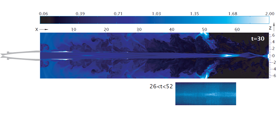
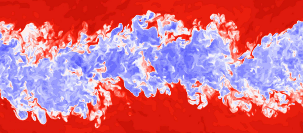
	Numerical simulation of an hypersonic light jet at M=5 with an initial density ratio between the external ambient and the jet equal to 10. The figure shows the density distribution at t=36. The flow is from left to right (see Tordella et al., DLES 7, 2010).
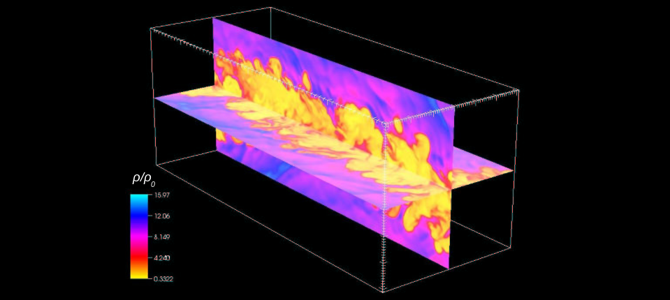
	Numerical simulation of an hypersonic light jet at M=5 with an initial density ratio between the external ambient and the jet equal to 10. The figure shows the density distribution in a longitudinal plane at t=32. The flow is from left to right (see Tordella et al., DLES 7, 2010).
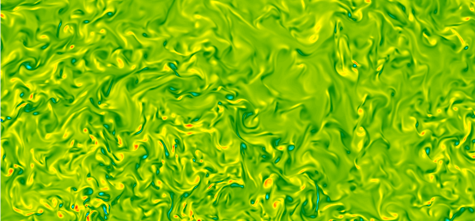
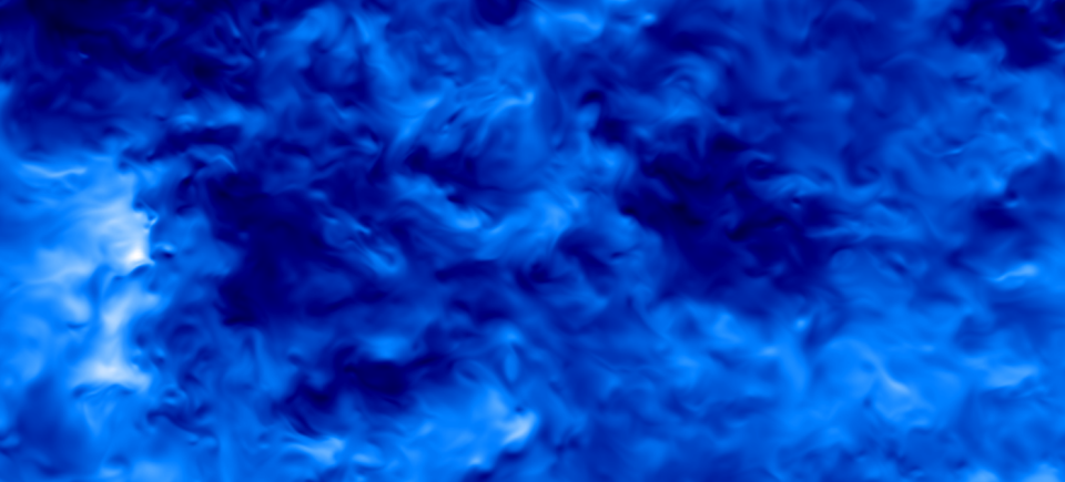
	Homogeneous and isotropic turbulence, Reλ=230: snapshot of the vorticity component in the direction normal to the figure.
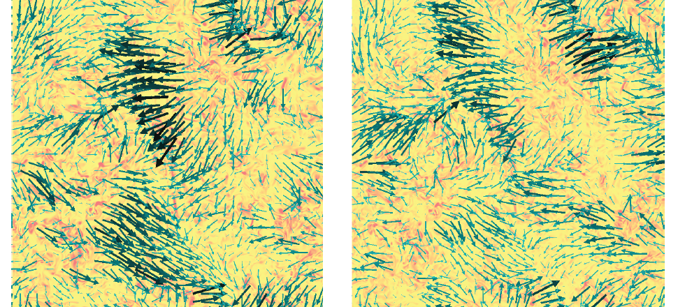
	Homogeneous and isotropic turbulence, Reλ=230. Arrows: Black: velocity field, Colours: enstrophy.
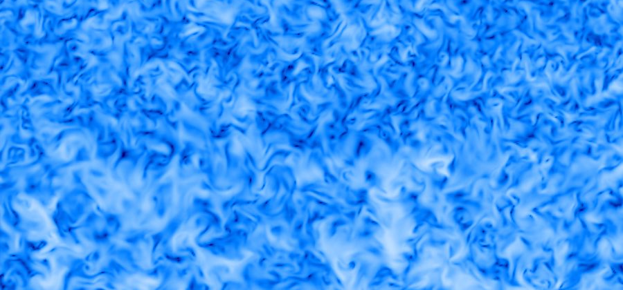
	Normalized stretching f (see Tordella et al., Comput. Phys. Comm. 141, 2007) in homogeneous and isotropic turbulence at Reλ=230.
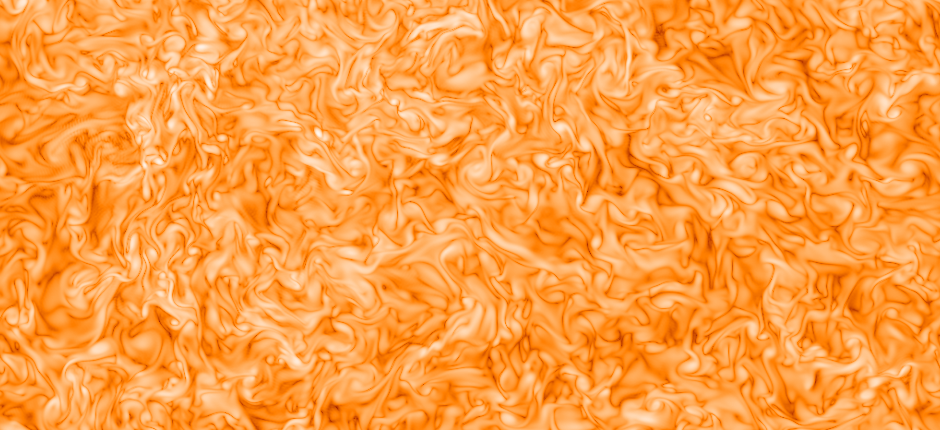
	Visualization of the velocity component normal to the plane of the figure in a turbulent flow at Reλ=230.
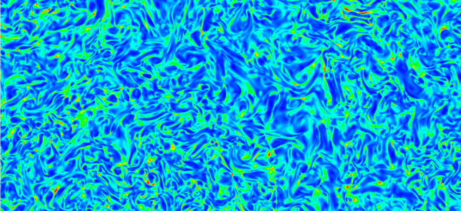
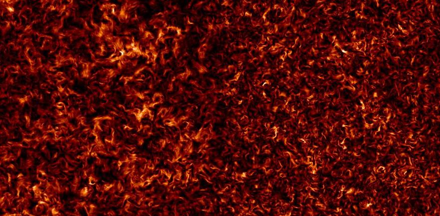
	Homogeneous and isotropic turbulence, Reλ=230: snapshot of the enstrophy distribution in logaritmic scale (lighter colours indicate higher values).
	Kinetic energy distribution in a shearless mixing in presence of a gradient of integral scale (see Tordella-Iovieno Physica D 142, 2012).
	Kinetic energy in a shearless mixing. The two regions (upper and lower half of the visualization) have the same integral scale but a different level of kinetic energy (see Tordella-Iovieno Phys.Rev.Lett. 107, 2011).
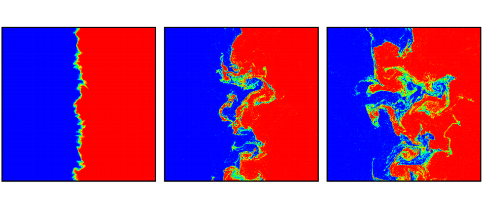
	Diffusion of a passive scalar across the interface which separates two homogeneous and isotropic regions with different energy in 2D turbulence. The visualization shows the scalar field in the central part of the computational domain. The high turbulent energy velocity field is on the left of each image. The three different instants correspond, from left to right, to t/τ = 1, 5, 10, respectively. τ is the initial eddy turnover time of the high energy region. (see Iovieno et al., J. Physics: Conf. Series 318, 2011).
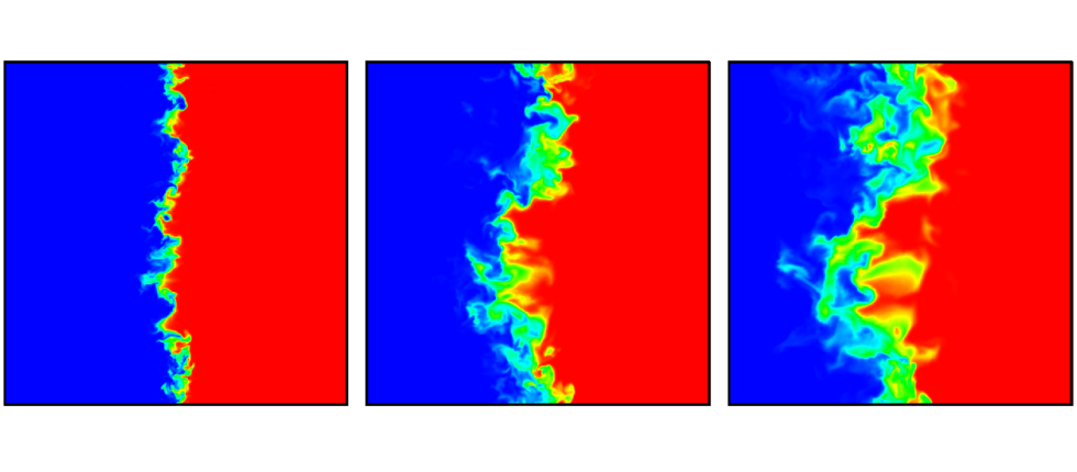
	Diffusion of a passive scalar across the interface which separates two homogeneous and isotropic regions with different energy. The visualization shows the scalar field in the central part of the computational domain. The high turbulent energy velocity field is on the left of each image. The three different instants correspond, from left to right, to t/τ = 1, 5, 10, respectively. τ is the initial eddy turnover time of the high energy region. This three-dimensional direct numerical simulation has an initial Reλ equal to 150 in the high energy isotropic region and 60 in the low energy region (see Iovieno et al., J. Physics: Conf. Series 318, 2011).
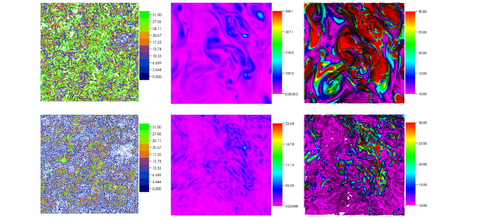
	Visualization of the vorticity magnitude in a section of the domain after having applied differend band filters (see Tordella et al., Physica D 284, 2014).
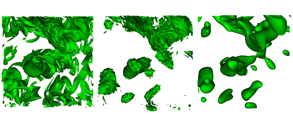
	Three dimensional visualization of the surfaces where one vorticity component has the nondimensional value 17.5 in a homogeneos turbulent flow with Reλ = 280. From left to right: unfiltered field; the wave number range 30–150 is filtered out by using the band-stop cross filter; the wave number range 30-infinity is filtered out by using the low-pass cross filter, i.e. by letting kMAX → ∞, see Eq. (5). The visualization shows a 2563 portion of the numerical field simulated on a 10243 mesh (see Tordella et al., Physica D 284, 2014).
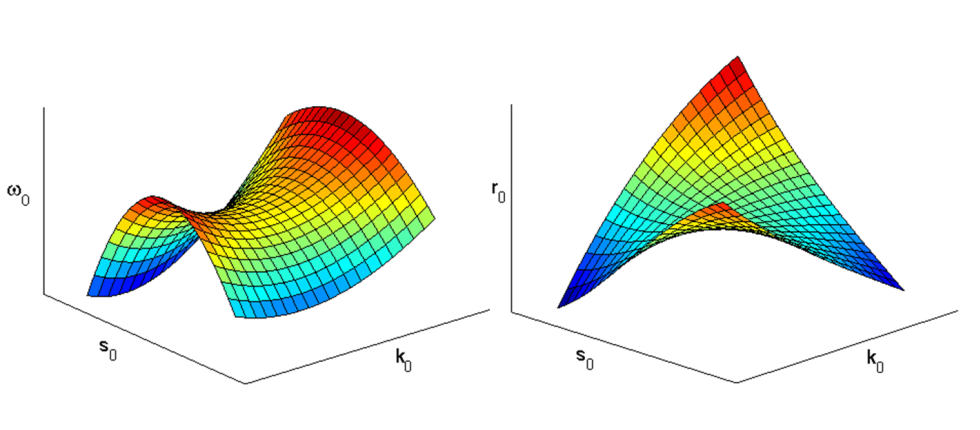
	Bluff-body wake. Saddle points multidimensional map: (a) ω0(k0,s0) and (b) r0(k0,s0), Re=35, 4 diameters downstream the body.
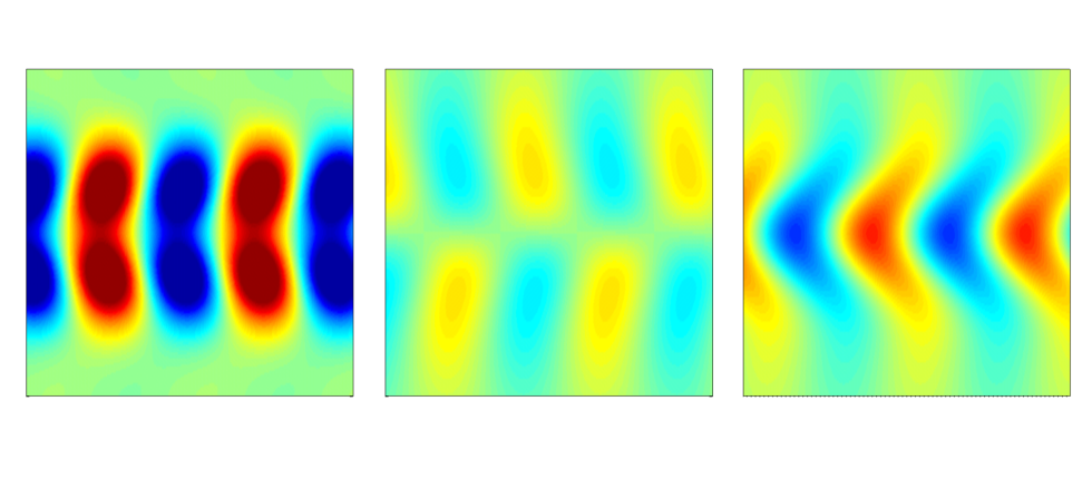
	Wake flow. Projection view visualizations of the perturbation velocity field in the physical plane (x, y), Re = 100, wake section: 50 body lengths downstream, t = 45°, angle of obliquity φ = 3/8 π, antisymmetric initial condition, k = 0.7. From left to right: u, v, w velocity components. The wavelength is normalized over the flow external spatial scale, the bluff body diameter D. The time is normalized over the flow relevant eddy turnover time, D/Uf, where Uf is the free stream velocity.
	Wake flow. Three dimensional plot of the velocity perturbation for a channel flow and a wake.
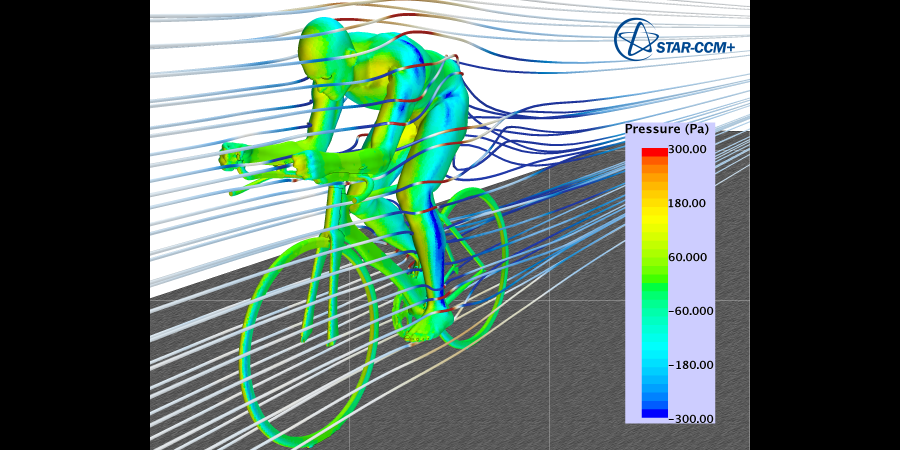
	Three-dimensional U-RANS (k-Omega SST model) of the flow around a bicycle (by Flavio Cimolin, CD-Adapco): streamlines and pressure on the cyclist/bicycle.