
Hydrodynamic Stability 1
- Details
- Last Updated on Sunday, 20 December 2015 15:36
Transient dynamics of three-dimensional perturbations
We consider an initial-value problem (IVP) for arbitrary small three-dimensional perturbations imposed on basic shear flows. We analyze three typical shear flows: the plane Poiseuille and Couette channel flows, the two-dimensional bluff-body wake, and the two- and three-dimensional boundary layer flows.
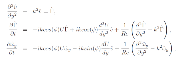
The viscous perturbation equations are combined in terms of the vorticity and velocity to obtain the Orr-Sommerfeld and the Squire equations. The first one is expressed in term of the transversal velocity laplacian and combined with a kinematics equation.
The equations are solved by means of a combined Fourier-Fourier (channel) and Laplace-Fourier (wake and boundary layer) transform in the plane normal to the basic flow. In the case of the channel flow, the dependent variables are in fact Fourier-Fourier transformed in the streamwise (x) and the spanwise (z) directions, which are both field homogeneity directions, while, in the case of the wake and the boundary layer flows, the variables are Fourier transformed along z, the only homogeneous direction of the system, and Laplace transformed along x (0 < x <∞).
Afterward, the resulting partial differential equations are numerically solved by the method of lines: the equations are first uniformly discretized in the spatial domain and then integrated in time. The spatial derivatives are discretized using a second-order finite difference scheme for the first and second derivatives. One-sided differences are adopted at the boundaries, while central differenced derivatives are used in the remaining part of the domain. The equations are then integrated in time by means of an adaptative one-step solver, based on an explicit Runge-Kutta (2,3) formula and implemented in the ode23 Matlab function. The choice of the ode23 routine is a good compromise between nonstiff solvers (ode45 and ode113), which give a higher order of accuracy, and stiff solvers (ode15s and ode23s), which can in general be more efficient.
Software Development
- Couette and Poiseuille plane channel flows [DOWNLOAD]
- Plane Wake flow [DOWNLOAD]
- 2D and 3D Boundary Layers flows [DOWNLOAD]
The structure of the numerical code is sketched in the following figure and the details of the Matlab scripts are given below.
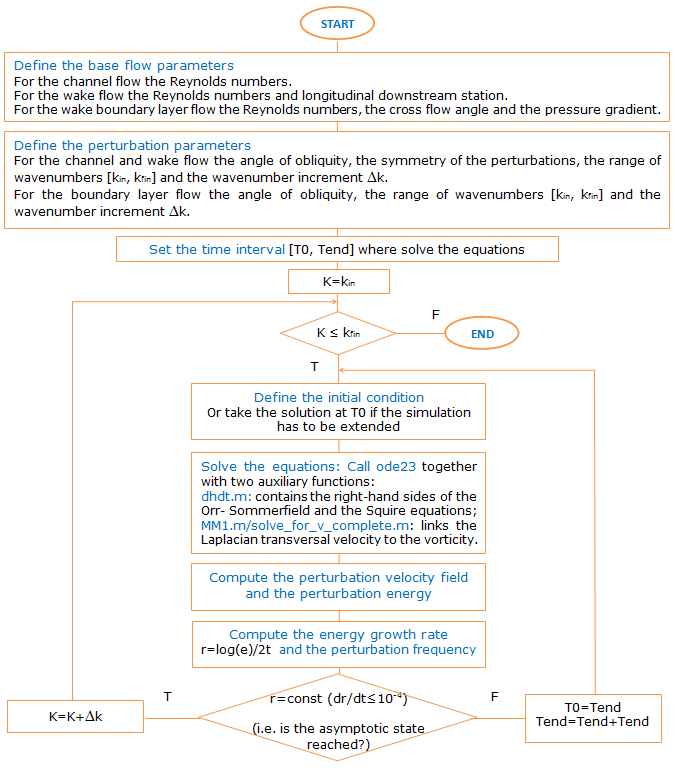
Figure 1. Flowchart of the Matlab codes.
- Channel_main.m/wake_main.m/BL_main.m: this file contains the main program necessary to use the code. The simulation parameters (angle of obliquity, symmetry of the perturbations, range of wavenumbers) are set as well as base flow configurations (Reynolds numbers and longitudinal downstream station for the wake flow) are set. A loop is defined which begins with the first simulated wavenumber, kin, and ends with the last simulated wavenumber, kfin. Once this cycle is entered, for a fixed wavenumber, the function IVP_complete.m is called;
- IVP_complete.m: the perturbative equations (1)-(3) are solved in this routine. Once the initial conditions are defined, the ode23 function is iteratively called together with three auxiliary functions, dhdt.m, MM1.m and solve_for_v_complete.m. The dhdt.m script represents the right-hand side of the perturbative equations (2)-(3), while MM1.m and solve_for_v_complete.m link the solutions of Eq. (1) to (2) (MM1.m is called for the channel and the boundary layer flows, solve_for_v_complete.m for the wake flow). Once the solutions are obtained, the perturbation velocity field and energy are computed, and verify_condition.m is called;
- verify_condition.m: this function verifies if the asymptotic condition for the current perturbative wave is reached. If the asymptotic state is not reached, IVP_complete.m is called again and the equations are further integrated in time. If the perturbation is instead in its asymptotic condition, the loop on the wavenumber range is incremented by one and the next wavenumber will be processed by channel_main.m/wake_main.m.
When the last selected wavenumber, kfin, verifies the asymptotic condition, the procedure stops.
More detailed notes on the initial-value problem formulation, numerical methods and the structure of the Matlab codes can be found here.